Let their probabilities and the corresponding conditional probabilities be known. Then the probability of the event occurring is:

This formula is called total probability formulas. In textbooks, it is formulated by a theorem, the proof of which is elementary: according to event algebra, (event happened And or an event happened And after it came the event or an event happened And after it came the event or …. or an event happened And event followed). Since the hypotheses are incompatible, and the event is dependent, then addition theorem for the probabilities of incompatible events (first step) And the theorem of multiplication of probabilities of dependent events (second step):

Probably, many anticipate the content of the first example =)

Wherever you spit - everywhere the urn:

Task 1

There are three identical urns. The first urn contains 4 white and 7 black balls, the second urn contains only white balls, and the third urn contains only black balls. One urn is chosen at random and a ball is drawn from it at random. What is the probability that this ball is black?

Solution: consider the event - a black ball will be drawn from a randomly selected urn. This event may or may not occur as a result of one of the following hypotheses:
– the 1st urn will be selected;
– the 2nd urn will be chosen;
– the 3rd urn will be chosen.

Since the urn is chosen at random, the choice of any of the three urns equally possible, hence:

Note that the above hypotheses form full group of events, that is, according to the condition, a black ball can appear only from these urns, and for example, not fly from a billiard table. Let's do a simple intermediate check:
OK, let's move on:

The first urn contains 4 white + 7 black = 11 balls, each classical definition:
is the probability of drawing a black ball given that that the 1st urn will be selected.

The second urn contains only white balls, so if chosen the appearance of a black ball becomes impossible: .

And, finally, in the third urn there are only black balls, which means that the corresponding conditional probability extraction of the black ball will be (event is certain).

is the probability that a black ball will be drawn from a randomly selected urn.

Answer:

The analyzed example again suggests how important it is to UNDERSTAND THE CONDITION. Let's take the same problems with urns and balls - with their external similarity, the methods of solving can be completely different: somewhere it is required to apply only classical definition of probability, somewhere events independent, somewhere dependent, and somewhere we are talking about hypotheses. At the same time, there is no clear formal criterion for choosing a solution path - you almost always need to think about it. How to improve your skills? We solve, we solve and we solve again!

Task 2

There are 5 different rifles in the shooting range. The probabilities of hitting the target for a given shooter are respectively equal to 0.5; 0.55; 0.7; 0.75 and 0.4. What is the probability of hitting the target if the shooter fires one shot from a randomly selected rifle?

Short solution and answer at the end of the lesson.

In most thematic problems, the hypotheses are, of course, not equally probable:

Task 3

There are 5 rifles in the pyramid, three of which are equipped with an optical sight. The probability that the shooter will hit the target when fired from a rifle with a telescopic sight is 0.95; for a rifle without a telescopic sight, this probability is 0.7. Find the probability that the target will be hit if the shooter fires one shot from a rifle taken at random.

Solution: in this problem, the number of rifles is exactly the same as in the previous one, but there are only two hypotheses:
- the shooter will choose a rifle with an optical sight;
- the shooter will select a rifle without a telescopic sight.
By classical definition of probability: .
Control:

Consider the event: - the shooter hits the target with a randomly selected rifle.
By condition: .

According to the total probability formula:

Answer: 0,85

In practice, a shortened way of designing a task, which you are also familiar with, is quite acceptable:

Solution: according to the classical definition: are the probabilities of choosing a rifle with and without an optical sight, respectively.

By condition, – probabilities of hitting the target with the respective types of rifles.

According to the total probability formula:
is the probability that the shooter will hit the target with a randomly selected rifle.

Answer: 0,85

Next task for independent decision:

Task 4

The engine operates in three modes: normal, forced and idling. In idle mode, the probability of its failure is 0.05, in normal mode - 0.1, and in forced mode - 0.7. 70% of the time the engine runs in normal mode, and 20% in forced mode. What is the probability of engine failure during operation?

Just in case, let me remind you - to get the probabilities, the percentages must be divided by 100. Be very careful! According to my observations, the conditions of problems for the total probability formula are often tried to be confused; and I specifically chose such an example. I'll tell you a secret - I almost got confused myself =)

Solution at the end of the lesson (formulated in a short way)

Problems for Bayes formulas

The material is closely related to the content of the previous paragraph. Let the event occur as a result of the implementation of one of the hypotheses . How to determine the probability that a particular hypothesis took place?

Given that that event already happened, probabilities of hypotheses overestimated according to the formulas that received the name of the English priest Thomas Bayes:

- the probability that the hypothesis took place;
- the probability that the hypothesis took place;
…
is the probability that the hypothesis was true.

At first glance, it seems like a complete absurdity - why recalculate the probabilities of hypotheses, if they are already known? But in fact there is a difference:

- This a priori(estimated before tests) probabilities.

- This a posteriori(estimated after tests) the probabilities of the same hypotheses, recalculated in connection with "newly discovered circumstances" - taking into account the fact that the event happened.

Let's look at this difference with a specific example:

Task 5

The warehouse received 2 batches of products: the first - 4000 pieces, the second - 6000 pieces. The average percentage of non-standard products in the first batch is 20%, and in the second - 10%. Randomly taken from the warehouse, the product turned out to be standard. Find the probability that it is: a) from the first batch, b) from the second batch.

First part solutions consists in using the total probability formula. In other words, the calculations are carried out under the assumption that the test not yet produced and event "the product turned out to be standard" until it comes.

Let's consider two hypotheses:
- a product taken at random will be from the 1st batch;
- a product taken at random will be from the 2nd batch.

Total: 4000 + 6000 = 10000 items in stock. According to the classical definition:
.

Control:

Consider the dependent event: – an item taken at random from the warehouse will standard.

In the first batch 100% - 20% = 80% standard products, therefore: given that that it belongs to the 1st party.

Similarly, in the second batch 100% - 10% = 90% standard products and is the probability that a randomly selected item in the warehouse will be a standard item given that that it belongs to the 2nd party.

According to the total probability formula:
is the probability that a product chosen at random from the warehouse will be a standard product.

Part two. Suppose that a product taken at random from the warehouse turned out to be standard. This phrase is directly spelled out in the condition, and it states the fact that the event happened.

According to Bayes' formulas:

a) - the probability that the selected standard product belongs to the 1st batch;

b) - the probability that the selected standard product belongs to the 2nd batch.

After revaluation hypotheses, of course, still form full group:
(examination;-))

Answer:

Ivan Vasilyevich, who changed his profession again and became the director of the plant, will help us understand the meaning of the reassessment of hypotheses. He knows that today the 1st shop shipped 4000 items to the warehouse, and the 2nd shop - 6000 products, and he comes to make sure of this. Suppose all products are of the same type and are in the same container. Naturally, Ivan Vasilyevich previously calculated that the product that he would now remove for verification would most likely be produced by the 1st workshop and with a probability by the second. But after the selected item turns out to be standard, he exclaims: “What a cool bolt! - it was rather released by the 2nd workshop. Thus, the probability of the second hypothesis is overestimated in better side, and the probability of the first hypothesis is underestimated: . And this overestimation is not unreasonable - after all, the 2nd workshop not only produced more products, but also works 2 times better!

You say, pure subjectivism? Partly - yes, moreover, Bayes himself interpreted a posteriori probabilities as trust level. However, not everything is so simple - there is an objective grain in the Bayesian approach. After all, the probability that the product will be standard (0.8 and 0.9 for the 1st and 2nd shops, respectively) This preliminary(a priori) and medium estimates. But, speaking philosophically, everything flows, everything changes, including probabilities. It is quite possible that at the time of the study more successful 2nd shop increased the percentage of standard products (and/or the 1st shop reduced), and if you check more or all 10 thousand items in stock, then the overestimated values ​​will be much closer to the truth.

By the way, if Ivan Vasilyevich extracts a non-standard part, then vice versa - he will “suspect” the 1st shop more and less - the second. I suggest you check it out for yourself:

Task 6

The warehouse received 2 batches of products: the first - 4000 pieces, the second - 6000 pieces. The average percentage of non-standard products in the first batch is 20%, in the second - 10%. A product taken at random from the warehouse turned out to be Not standard. Find the probability that it is: a) from the first batch, b) from the second batch.

The condition will be distinguished by two letters, which I have highlighted in bold. The problem can be solved from scratch, or you can use the results of previous calculations. In the sample I have complete solution, but so that there is no formal overlap with Task No. 5, the event “A product taken at random from the warehouse will be non-standard” marked with .

The Bayesian scheme of re-evaluation of probabilities is found everywhere, and it is also actively exploited by various kinds of scammers. Consider a three-letter joint-stock company that has become a household name, which attracts deposits from the population, supposedly invests them somewhere, regularly pays dividends, etc. What's happening? Day after day, month after month passes, and more and more new facts, conveyed through advertising and word of mouth, only increase the level of confidence in the financial pyramid (posterior Bayesian re-evaluation due to past events!). That is, in the eyes of depositors, there is a constant increase in the likelihood that "this is a serious office"; while the probability of the opposite hypothesis (“these are regular scammers”), of course, decreases and decreases. The rest, I think, is clear. It is noteworthy that the earned reputation gives the organizers time to successfully hide from Ivan Vasilyevich, who was left not only without a batch of bolts, but also without pants.

We will return to no less interesting examples a little later, but for now, perhaps the most common case with three hypotheses is next in line:

Task 7

Electric lamps are manufactured at three factories. The 1st plant produces 30% of the total number of lamps, the 2nd - 55%, and the 3rd - the rest. The products of the 1st plant contain 1% of defective lamps, the 2nd - 1.5%, the 3rd - 2%. The store receives products from all three factories. The lamp I bought was defective. What is the probability that it was produced by plant 2?

Note that in problems on Bayes formulas in the condition Necessarily some what happened an event, in this case, the purchase of a lamp.

Events have increased and solution it is more convenient to arrange in a "fast" style.

The algorithm is exactly the same: at the first step, we find the probability that the purchased lamp will will be defective.

Using the initial data, we translate the percentages into probabilities:
are the probabilities that the lamp is produced by the 1st, 2nd and 3rd factories, respectively.
Control:

Similarly: - the probabilities of manufacturing a defective lamp for the respective factories.

According to the total probability formula:

- the probability that the purchased lamp will be defective.

Step two. Let the purchased lamp be defective (the event happened)

According to the Bayes formula:
- the probability that the purchased defective lamp is manufactured by a second factory

Answer:

Why did the initial probability of the 2nd hypothesis increase after the reassessment? After all, the second plant produces lamps of average quality (the first one is better, the third one is worse). So why did it increase a posteriori the probability that the defective lamp is from the 2nd factory? This is no longer due to "reputation", but to size. Since plant No. 2 produced the largest number of lamps, they blame it (at least subjectively): “most likely, this defective lamp is from there”.

It is interesting to note that the probabilities of the 1st and 3rd hypotheses were overestimated in the expected directions and became equal:

Control: , which was to be verified.

By the way, about underestimated and overestimated:

Task 8

IN student group 3 people have a high level of training, 19 people have an average level and 3 people have a low level. Probabilities successful delivery exam for these students are respectively equal to: 0.95; 0.7 and 0.4. It is known that some student passed the exam. What is the probability that:

a) he was very well prepared;
b) was moderately prepared;
c) was poorly prepared.

Perform calculations and analyze the results of reevaluation of hypotheses.

The task is close to reality and is especially plausible for a group of part-time students, where the teacher practically does not know the abilities of this or that student. In this case, the result can cause rather unexpected consequences. (especially for exams in the 1st semester). If an ill-prepared student is lucky enough to get a ticket, then the teacher is likely to consider him a good student or even a strong student, which will bring good dividends in the future (of course, you need to “raise the bar” and maintain your image). If a student studied, crammed, repeated for 7 days and 7 nights, but he was simply unlucky, then further events can develop in the worst possible way - with numerous retakes and balancing on the verge of departure.

Needless to say, reputation is the most important capital, it is no coincidence that many corporations bear the names and surnames of their founding fathers, who led the business 100-200 years ago and became famous for their impeccable reputation.

Yes, the Bayesian approach to some extent subjective, but ... that's how life works!

Let's consolidate the material with a final industrial example, in which I will talk about the technical subtleties of the solution that have not yet been encountered:

Task 9

Three workshops of the plant produce parts of the same type, which are assembled in a common container for assembly. It is known that the first shop produces 2 times more parts than the second shop, and 4 times more than the third shop. In the first workshop, the defect is 12%, in the second - 8%, in the third - 4%. For control, one part is taken from the container. What is the probability that it will be defective? What is the probability that the extracted defective part was produced by the 3rd workshop?

Taki Ivan Vasilyevich is on horseback again =) The film must have a happy ending =)

Solution: in contrast to Tasks No. 5-8, a question is explicitly asked here, which is resolved using the total probability formula. But on the other hand, the condition is a little “encrypted”, and the school skill to compose the simplest equations will help us solve this rebus. For "x" it is convenient to take the smallest value:

Let be the share of parts produced by the third workshop.

According to the condition, the first workshop produces 4 times more than the third workshop, so the share of the 1st workshop is .

In addition, the first workshop produces 2 times more products than the second workshop, which means that the share of the latter: .

Let's make and solve the equation:

Thus: - the probabilities that the part removed from the container was released by the 1st, 2nd and 3rd workshops, respectively.

Control: . In addition, it will not be superfluous to look again at the phrase “It is known that the first workshop produces products 2 times more than the second workshop and 4 times more than the third workshop” and make sure that the obtained probabilities really correspond to this condition.

For "X" it was initially possible to take the share of the 1st or the share of the 2nd shop - the probabilities will come out the same. But, one way or another, the most difficult section has been passed, and the solution is on track:

From the condition we find:
- the probability of manufacturing a defective part for the corresponding workshops.

According to the total probability formula:
is the probability that a part randomly extracted from the container will be non-standard.

Question two: what is the probability that the extracted defective part was produced by the 3rd workshop? This question assumes that the part has already been removed and is found to be defective. We reevaluate the hypothesis using the Bayes formula:
is the desired probability. Quite expected - after all, the third workshop produces not only the smallest share of parts, but also leads in quality!

In this case, I had to simplify the four-story fraction, which in problems on Bayes formulas has to be done quite often. But for this lesson, I somehow accidentally picked up examples in which many calculations can be done without ordinary fractions.

Since there are no “a” and “be” points in the condition, it is better to provide the answer with text comments:

Answer: - the probability that the part removed from the container will be defective; - the probability that the extracted defective part was released by the 3rd workshop.

As you can see, the problems on the total probability formula and Bayes formulas are quite simple, and, probably, for this reason they so often try to complicate the condition, which I already mentioned at the beginning of the article.

Additional examples are in the file with ready-made solutions for F.P.V. and Bayes formulas, in addition, there are probably those who wish to become more deeply acquainted with this topic in other sources. And the topic is really very interesting - what is it worth alone bayes paradox, which justifies the everyday advice that if a person is diagnosed with a rare disease, then it makes sense for him to conduct a second and even two repeated independent examinations. It would seem that they do it solely out of desperation ... - but no! But let's not talk about sad things.

is the probability that a randomly selected student will pass the exam.
Let the student pass the exam. According to Bayes' formulas:
A) - the probability that the student who passed the exam was prepared very well. The objective initial probability is overestimated, because almost always some "average" are lucky with questions and they answer very strongly, which gives the erroneous impression of impeccable preparation.
b) is the probability that the student who passed the exam was moderately prepared. The initial probability turns out to be slightly overestimated, because students with an average level of preparation are usually the majority, in addition, the teacher will include unsuccessfully answered “excellent students” here, and occasionally a poorly performing student who was very lucky with a ticket.
V) - the probability that the student who passed the exam was poorly prepared. The initial probability was overestimated for the worse. Not surprising.
Examination:
Answer : Bayes formula:

The probabilities P(H i) of the hypotheses H i are called a priori probabilities - the probabilities before the experiments.
The probabilities P(A/H i) are called a posteriori probabilities - the probabilities of the hypotheses H i refined as a result of the experiment.

Example #1. The device can be assembled from high quality parts and from parts of ordinary quality. About 40% of devices are assembled from high quality parts. If the device is assembled from high-quality parts, its reliability (probability of failure-free operation) over time t is 0.95; if from parts of ordinary quality - its reliability is 0.7. The device was tested for time t and worked flawlessly. Find the probability that it is assembled from high quality parts.
Solution. Two hypotheses are possible: H 1 - the device is assembled from high-quality parts; H 2 - the device is assembled from parts of ordinary quality. The probabilities of these hypotheses before the experiment: P(H 1) = 0.4, P(H 2) = 0.6. As a result of the experiment, event A was observed - the device worked flawlessly for time t. Conditional probabilities of this event under hypotheses H 1 and H 2 are: P(A|H 1) = 0.95; P(A|H 2) = 0.7. Using formula (12), we find the probability of the hypothesis H 1 after the experiment:

Example #2. Two shooters independently shoot at one target, each firing one shot. The probability of hitting the target for the first shooter is 0.8, for the second 0.4. After shooting, one hole was found in the target. Assuming that two shooters cannot hit the same point, find the probability that the first shooter hit the target.
Solution. Let event A be one hole found in the target after shooting. Before the start of the shooting, hypotheses are possible:
H 1 - neither the first nor the second shooter will hit, the probability of this hypothesis: P(H 1) = 0.2 0.6 = 0.12.
H 2 - both shooters will hit, P(H 2) = 0.8 0.4 = 0.32.
H 3 - the first shooter will hit, and the second will not hit, P(H 3) = 0.8 0.6 = 0.48.
H 4 - the first shooter will not hit, but the second will hit, P (H 4) = 0.2 0.4 = 0.08.
The conditional probabilities of the event A under these hypotheses are:

After experience, the hypotheses H 1 and H 2 become impossible, and the probabilities of the hypotheses H 3 and H 4
will be equal:

So, it is most likely that the target is hit by the first shooter.

Example #3. In the assembly shop, an electric motor is connected to the device. Electric motors are supplied by three manufacturers. There are 19.6 and 11 electric motors of the named plants in the warehouse, respectively, which can work without failure until the end of the warranty period, respectively, with probabilities of 0.85, 0.76 and 0.71. The worker randomly takes one engine and mounts it to the device. Find the probability that the electric motor, mounted and working without fail until the end of the warranty period, was supplied by the first, second or third manufacturer, respectively.
Solution. The first test is the choice of the electric motor, the second is the operation of the electric motor during the warranty period. Consider the following events:
A - the electric motor works flawlessly until the end of the warranty period;
H 1 - the fitter will take the engine from the products of the first plant;
H 2 - the fitter will take the engine from the products of the second plant;
H 3 - the fitter will take the engine from the products of the third plant.
The probability of event A is calculated by the total probability formula:

Conditional probabilities are specified in the problem statement:

Let's find the probabilities

Using the Bayes formulas (12), we calculate the conditional probabilities of the hypotheses H i:

Example #4. The probabilities that during the operation of the system, which consists of three elements, the elements with numbers 1, 2 and 3 will fail, are related as 3: 2: 5. The probabilities of detecting failures of these elements are 0.95, respectively; 0.9 and 0.6.

b) Under the conditions of this task, a failure was detected during the operation of the system. Which element is most likely to fail?

Solution.
Let A be a failure event. Let us introduce a system of hypotheses H1 - failure of the first element, H2 - failure of the second element, H3 - failure of the third element.
We find the probabilities of hypotheses:
P(H1) = 3/(3+2+5) = 0.3
P(H2) = 2/(3+2+5) = 0.2
P(H3) = 5/(3+2+5) = 0.5

According to the condition of the problem, the conditional probabilities of event A are:
P(A|H1) = 0.95, P(A|H2) = 0.9, P(A|H3) = 0.6

a) Find the probability of detecting a failure in the system.
P(A) = P(H1)*P(A|H1) + P(H2)*P(A|H2) + P(H3)*P(A|H3) = 0.3*0.95 + 0.2*0.9 + 0.5 *0.6 = 0.765

b) Under the conditions of this task, a failure was detected during the operation of the system. Which element is most likely to fail?
P1 = P(H1)*P(A|H1)/ P(A) = 0.3*0.95 / 0.765 = 0.373
P2 = P(H2)*P(A|H2)/ P(A) = 0.2*0.9 / 0.765 = 0.235
P3 = P(H3)*P(A|H3)/ P(A) = 0.5*0.6 / 0.765 = 0.392

The maximum probability of the third element.

Who is Bayes? And what does it have to do with management? – may be followed by quite a fair question. For now, take my word for it: this is very important! .. and interesting (at least for me).

What paradigm do most managers operate in: if I observe something, what conclusions can I draw from it? What does Bayes teach: what must actually be in order for me to observe this something? This is how all sciences develop, and he writes about this (I quote from memory): a person who does not have a theory in his head will shy away from one idea to another under the influence of various events (observations). Not for nothing they say: there is nothing more practical than a good theory.

An example from practice. My subordinate makes a mistake, and my colleague (the head of another department) says that it would be necessary to exert managerial influence on the negligent employee (in other words, punish / scold). And I know that this employee makes 4-5 thousand of the same type of operations per month, and during this time he makes no more than 10 mistakes. Feel the difference in the paradigm? My colleague reacts to observation, and I have a priori knowledge that an employee makes a certain number of mistakes, so another one did not affect this knowledge ... Now, if at the end of the month it turns out that there are, for example, 15 such errors! .. This will already become a reason to investigate the causes of non-compliance with standards.

Convinced of the importance of the Bayesian approach? Intrigued? Hope so". And now a fly in the ointment. Unfortunately, Bayesian ideas are rarely given on the first go. I was frankly unlucky, as I got acquainted with these ideas through popular literature, after reading which many questions remained. When planning to write a note, I collected everything that I had previously outlined according to Bayes, and also studied what they write on the Internet. I present to you my best guess on the subject. Introduction to Bayesian Probability.

Derivation of Bayes' theorem

Consider the following experiment: we call any number lying on the segment and fix when this number is, for example, between 0.1 and 0.4 (Fig. 1a). The probability of this event is equal to the ratio of the length of the segment to the total length of the segment, provided that the occurrence of numbers on the segment equiprobable. Mathematically, this can be written p(0,1 <= x <= 0,4) = 0,3, или кратко R(X) = 0.3, where R- probability, X is a random variable in the range , X is a random variable in the range . That is, the probability of hitting the segment is 30%.

Rice. 1. Graphical interpretation of probabilities

Now consider the square x (Fig. 1b). Let's say we have to name pairs of numbers ( x, y), each of which is greater than zero and less than one. The probability that x(first number) will be within the segment (blue area 1), equal to the ratio of the area of ​​​​the blue area to the area of ​​\u200b\u200bthe entire square, that is, (0.4 - 0.1) * (1 - 0) / (1 * 1) = 0, 3, that is, the same 30%. The probability that y is inside the segment (green area 2) is equal to the ratio of the area of ​​the green area to the area of ​​the entire square p(0,5 <= y <= 0,7) = 0,2, или кратко R(Y) = 0,2.

What can be learned about the values ​​at the same time x And y. For example, what is the probability that both x And y are in the corresponding given segments? To do this, you need to calculate the ratio of the area of ​​\u200b\u200bdomain 3 (the intersection of the green and blue stripes) to the area of ​​the entire square: p(X, Y) = (0,4 – 0,1) * (0,7 – 0,5) / (1 * 1) = 0,06.

Now suppose we want to know what is the probability that y is in the interval if x is already in the range. That is, in fact, we have a filter and when we call pairs ( x, y), then we immediately discard those pairs that do not satisfy the condition for finding x in a given interval, and then from the filtered pairs we count those for which y satisfies our condition and consider the probability as the ratio of the number of pairs for which y lies in the above segment to the total number of filtered pairs (that is, for which x lies in the segment). We can write this probability as p(Y|X at X hit in the range." Obviously, this probability is equal to the ratio of the area of ​​area 3 to the area of ​​blue area 1. The area of ​​area 3 is (0.4 - 0.1) * (0.7 - 0.5) = 0.06, and the area of ​​blue area 1 ( 0.4 - 0.1) * (1 - 0) = 0.3, then their ratio is 0.06 / 0.3 = 0.2. In other words, the probability of finding y on the segment, provided that x belongs to the segment p(Y|X) = 0,2.

In the previous paragraph, we actually formulated the identity: p(Y|X) = p(X, Y) /p( X). It reads: "probability of hitting at in the range, provided that X hit in the range is equal to the ratio of the probability of simultaneous hit X in range and at in the range, to the probability of hitting X into the range."

By analogy, consider the probability p(X|Y). We call couples x, y) and filter those for which y lies between 0.5 and 0.7, then the probability that x is in the segment provided that y belongs to the segment is equal to the ratio of the area of ​​area 3 to the area of ​​green area 2: p(X|Y) = p(X, Y) / p(Y).

Note that the probabilities p(X, Y) And p(Y, X) are equal, and both are equal to the ratio of the area of ​​zone 3 to the area of ​​the entire square, but the probabilities p(Y|X) And p(X|Y) not equal; while the probability p(Y|X) is equal to the ratio of the area of ​​area 3 to area 1, and p(X|Y) – domain 3 to domain 2. Note also that p(X, Y) is often denoted as p(X&Y).

So we have two definitions: p(Y|X) = p(X, Y) /p( X) And p(X|Y) = p(X, Y) / p(Y)

Let's rewrite these equalities as: p(X, Y) = p(Y|X)*p( X) And p(X, Y) = p(X|Y) * p(Y)

Since the left sides are equal, so are the right ones: p(Y|X)*p( X) = p(X|Y) * p(Y)

Or we can rewrite the last equality as:

This is Bayes' theorem!

Is it possible that such simple (almost tautological) transformations give rise to a great theorem!? Do not rush to conclusions. Let's talk again about what we got. There was some initial (a priori) probability R(X) that the random variable X uniformly distributed on the segment falls within the range X. Some event has happened Y, as a result of which we have obtained the a posteriori probability of the same random variable X: R(X|Y), and this probability differs from R(X) by the coefficient . Event Y called evidence, more or less confirming or refuting X. This coefficient is sometimes called power of evidence. The stronger the evidence, the more the fact of observation Y changes the prior probability, the more the posterior probability differs from the prior. If the evidence is weak, the posterior is nearly equal to the prior.

Bayes formula for discrete random variables

In the previous section, we derived the Bayes formula for continuous random variables x and y defined on the interval . Consider an example with discrete random variables, each taking on two possible values. In the course of routine medical examinations, it was found that at the age of forty, 1% of women suffer from breast cancer. 80% of women with cancer get positive mammography results. 9.6% of healthy women also get positive mammography results. During the examination, a woman of this age group received a positive mammogram result. What is the probability that she actually has breast cancer?

The course of reasoning/calculations is as follows. Of the 1% of cancer patients, mammography will give 80% positive results = 1% * 80% = 0.8%. Of 99% of healthy women, mammography will give 9.6% positive results = 99% * 9.6% = 9.504%. In total, out of 10.304% (9.504% + 0.8%) with positive mammogram results, only 0.8% are sick, and the remaining 9.504% are healthy. Thus, the probability that a woman with a positive mammogram has cancer is 0.8% / 10.304% = 7.764%. Did you think 80% or so?

In our example, the Bayes formula takes the following form:

Let's talk about the "physical" meaning of this formula once again. X is a random variable (diagnosis), which takes the following values: X 1- sick and X 2- healthy; Y– random variable (measurement result - mammography), which takes the values: Y 1- a positive result and Y2- negative result; p(X 1)- the probability of illness before mammography (a priori probability), equal to 1%; R(Y 1 |X 1 ) – the probability of a positive result if the patient is sick (conditional probability, since it must be specified in the conditions of the task), equal to 80%; R(Y 1 |X 2 ) – the probability of a positive result if the patient is healthy (also conditional probability), equal to 9.6%; p(X 2)- the probability that the patient is healthy before mammography (a priori probability), equal to 99%; p(X 1|Y 1 ) – the probability that the patient is ill, given a positive mammogram result (posterior probability).

It can be seen that the posterior probability (what we are looking for) is proportional to the prior probability (initial) with a slightly more complex coefficient . I will emphasize again. In my opinion, this is a fundamental aspect of the Bayesian approach. Dimension ( Y) added a certain amount of information to the initially available (a priori), which clarified our knowledge about the object.

Examples

To consolidate the material covered, try to solve several problems.

Example 1 There are 3 urns; in the first 3 white balls and 1 black; in the second - 2 white balls and 3 black ones; in the third - 3 white balls. Someone randomly approaches one of the urns and draws 1 ball from it. This ball is white. Find the posterior probabilities that the ball is drawn from the 1st, 2nd, 3rd urn.

Solution. We have three hypotheses: H 1 = (first urn selected), H 2 = (second urn selected), H 3 = (third urn selected). Since the urn is chosen at random, the a priori probabilities of the hypotheses are: Р(Н 1) = Р(Н 2) = Р(Н 3) = 1/3.

As a result of the experiment, the event A = appeared (a white ball was taken out of the selected urn). Conditional probabilities of event A under hypotheses H 1, H 2, H 3: P(A|H 1) = 3/4, P(A|H 2) = 2/5, P(A|H 3) = 1. For example , the first equality reads like this: “the probability of drawing a white ball if the first urn is chosen is 3/4 (since there are 4 balls in the first urn, and 3 of them are white)”.

Applying the Bayes formula, we find the posterior probabilities of the hypotheses:

Thus, in the light of information about the occurrence of event A, the probabilities of the hypotheses changed: the most probable became the hypothesis H 3 , the least probable - the hypothesis H 2 .

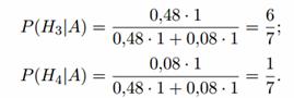
Example 2 Two shooters independently shoot at the same target, each firing one shot. The probability of hitting the target for the first shooter is 0.8, for the second - 0.4. After shooting, one hole was found in the target. Find the probability that this hole belongs to the first shooter (we discard the outcome (both holes coincided) as negligibly unlikely).

Solution. Before the experiment, the following hypotheses are possible: H 1 = (neither the first nor the second arrows will hit), H 2 = (both arrows will hit), H 3 - (the first shooter will hit, and the second will not), H 4 = (the first shooter will not will hit, and the second will hit). Prior probabilities of hypotheses:

P (H 1) \u003d 0.2 * 0.6 \u003d 0.12; P (H 2) \u003d 0.8 * 0.4 \u003d 0.32; P (H 3) \u003d 0.8 * 0.6 \u003d 0.48; P (H 4) \u003d 0.2 * 0.4 \u003d 0.08.

The conditional probabilities of the observed event A = (there is one hole in the target) under these hypotheses are: P(A|H 1) = P(A|H 2) = 0; P(A|H 3) = P(A|H 4) = 1

After experience, the hypotheses H 1 and H 2 become impossible, and the posterior probabilities of the hypotheses H 3 and H 4 according to the Bayes formula will be:

Bayes against spam

Bayes' formula has found wide application in the development of spam filters. Let's say you want to train a computer to determine which emails are spam. We will start from the dictionary and word combinations using Bayesian estimates. Let us first create a space of hypotheses. Let us have 2 hypotheses regarding any letter: H A is spam, H B is not spam, but a normal, necessary letter.

First, let's "train" our future anti-spam system. Let's take all the letters we have and divide them into two "heaps" of 10 letters. We put spam letters in one and call it the H A heap, in the other we put the necessary correspondence and call it the H B heap. Now let's see: what words and phrases are found in spam and necessary emails and with what frequency? These words and phrases will be called evidence and denoted by E 1 , E 2 ... It turns out that commonly used words (for example, the words “like”, “your”) in the heaps H A and H B occur with approximately the same frequency. Thus, the presence of these words in a letter tells us nothing about which heap it belongs to (weak evidence). Let's assign to these words a neutral value of the estimation of the probability of "spam", say, 0.5.

Let the phrase "conversational English" appear in only 10 letters, and more often in spam emails (for example, in 7 spam emails out of all 10) than in the right ones (in 3 out of 10). Let's give this phrase a higher score of 7/10 for spam, and a lower score for normal emails: 3/10. Conversely, it turned out that the word "buddy" was more common in normal letters (6 out of 10). And so we received a short letter: “Friend! How is your spoken English?. Let's try to evaluate its "spamness". We will put the general estimates P(H A), P(H B) of belonging to each heap using a somewhat simplified Bayes formula and our approximate estimates:

P(H A) = A/(A+B), Where A \u003d p a1 * p a2 * ... * pan, B \u003d p b1 * p b2 * ... * p b n \u003d (1 - p a1) * (1 - p a2) * ... * (1 - p an).

Table 1. Simplified (and incomplete) Bayesian evaluation of writing

Thus, our hypothetical letter received an assessment of the probability of belonging with an emphasis in the direction of "spam". Can we decide to throw the letter into one of the piles? Let's set the decision thresholds:

• We will assume that the letter belongs to the heap H i if P(H i) ≥ T.
• The letter does not belong to the heap if P(H i) ≤ L.
• If L ≤ P(H i) ≤ T, then no decision can be made.

You can take T = 0.95 and L = 0.05. Since for the letter in question and 0.05< P(H A) < 0,95, и 0,05 < P(H В) < 0,95, то мы не сможем принять решение, куда отнести данное письмо: к спаму (H A) или к нужным письмам (H B). Можно ли улучшить оценку, используя больше информации?

Yes. Let's calculate the score for each piece of evidence in a different way, just like Bayes suggested. Let be:

F a is the total number of spam emails;

F ai is the number of letters with a certificate i in a pile of spam;

F b is the total number of letters needed;

F bi is the number of letters with a certificate i in a pile of necessary (relevant) letters.

Then: p ai = F ai /F a , p bi = F bi /F b . P(H A) = A/(A+B), P(H B) = B/(A+B), WhereА = p a1 *p a2 *…*p an , B = p b1 *p b2 *…*p b n

Please note that the scores of evidence words p ai and p bi have become objective and can be calculated without human participation.

Table 2. A more accurate (but incomplete) Bayesian estimate for available features from a letter

We got a quite definite result - with a large margin of probability, the letter can be attributed to the necessary letters, since P(H B) = 0.997 > T = 0.95. Why did the result change? Because we used more information - we took into account the number of letters in each of the heaps and, by the way, determined the estimates p ai and p bi much more correctly. They were determined in the same way as Bayes himself did, by calculating the conditional probabilities. In other words, p a3 is the probability that the word "buddy" will appear in the email, given that the email already belongs to the spam heap H A . The result was not long in coming - it seems that we can make a decision with greater certainty.

Bayes vs Corporate Fraud

An interesting application of the Bayesian approach was described by MAGNUS8.

My current project (IS for detecting fraud in a manufacturing enterprise) uses the Bayes formula to determine the likelihood of fraud (fraud) in the presence / absence of several facts indirectly in favor of the hypothesis of the possibility of fraud. The algorithm is self-learning (with feedback), i.e. recalculates its coefficients (conditional probabilities) upon actual confirmation or non-confirmation of the fraud during the verification by the economic security service.

It is probably worth saying that such methods when designing algorithms require a fairly high mathematical culture of the developer, because the slightest error in the derivation and/or implementation of computational formulas will nullify and discredit the entire method. Probabilistic methods are especially guilty of this, since human thinking is not adapted to work with probabilistic categories and, accordingly, there is no “visibility” and understanding of the “physical meaning” of intermediate and final probabilistic parameters. Such an understanding exists only for the basic concepts of probability theory, and then you just need to very carefully combine and derive complex things according to the laws of probability theory - common sense will no longer help for composite objects. This, in particular, is associated with quite serious methodological battles that take place on the pages of modern books on the philosophy of probability, as well as a large number of sophisms, paradoxes and curiosities on this topic.

One more nuance that I had to face - unfortunately, almost everything more or less USEFUL IN PRACTICE on this topic is written in English. In Russian-language sources, there is basically only a well-known theory with demonstration examples only for the most primitive cases.

I fully agree with the last comment. For example, Google, when trying to find something like “Bayesian Probability” book, did not give anything intelligible. True, he said that a book with Bayesian statistics was banned in China. (Statistics professor Andrew Gelman reported on a Columbia University blog that his book, Data Analysis with Regression and Multilevel/Hierarchical Models, was banned from publication in China. text.”) I wonder if a similar reason led to the absence of books on Bayesian probability in Russia?

Conservatism in the process of human information processing

Probabilities determine the degree of uncertainty. Probability, both according to Bayes and our intuition, is simply a number between zero and what represents the degree to which a somewhat idealized person believes the statement is true. The reason why man is somewhat idealized is that the sum of his probabilities for two mutually exclusive events must equal his probability that either of those events will occur. The property of additivity has such implications that few real people can match them all.

Bayes' theorem is a trivial consequence of the property of additivity, undeniable and agreed upon by all probabilists, Bayesian and otherwise. One way to write it is the following. If P(H A |D) is the subsequent probability that hypothesis A was after the given value D was observed, P(H A) is its prior probability before the given value D was observed, P(D|H A ) is the probability that a given value D will be observed, if H A is true, and P(D) is the unconditional probability of a given value D, then

(1) P(H A |D) = P(D|H A) * P(H A) / P(D)

P(D) is best thought of as a normalizing constant causing the posterior probabilities to add up to one over the exhaustive set of mutually exclusive hypotheses that are being considered. If it needs to be calculated, it can be like this:

But more often P(D) is eliminated rather than counted. A convenient way to eliminate it is to transform Bayes' theorem into the form of a probability-odds relation.

Consider another hypothesis, H B , mutually exclusive to H A, and change your mind about it based on the same given quantity that changed your mind about H A. Bayes' theorem says that

(2) P(H B |D) = P(D|H B) * P(H B) / P(D)

Now we divide Equation 1 by Equation 2; the result will be like this:

where Ω 1 are the posterior odds in favor of H A in terms of H B , Ω 0 are the prior odds, and L is a number familiar to statisticians as a ratio of probabilities. Equation 3 is the same relevant version of Bayes' theorem as Equation 1, and is often much more useful especially for experiments involving hypotheses. Bayesian proponents argue that Bayes' theorem is a formally optimal rule for how to revise opinions in the light of new data.

We are interested in comparing the ideal behavior defined by Bayes' theorem with the actual behavior of people. To give you some idea of ​​what this means, let's try an experiment with you as the subject. This bag contains 1000 poker chips. I have two of these bags, one with 700 red and 300 blue chips, and the other with 300 red and 700 blue. I flipped a coin to determine which one to use. Thus, if our opinions are the same, your current probability of drawing a bag with more red chips is 0.5. Now, you randomly sample, returning after each token. In 12 chips, you get 8 red and 4 blue. Now, based on everything you know, what is the probability that a bag came up with more reds? It is clear that it is higher than 0.5. Please do not continue reading until you have recorded your rating.

If you look like a typical subject, your score falls between 0.7 and 0.8. If we did the corresponding calculation, however, the answer would be 0.97. Indeed, it is very rare for a person who has not previously been shown the influence of conservatism to come to such a high estimate, even if he was familiar with Bayes' theorem.

If the proportion of red chips in the bag is R, then the probability of getting r red chips and ( n-r) blue in n samples with return - p r (1–p)n–r. Thus, in a typical bag and poker chip experiment, if HA means that the proportion of red chips is r A And HB means that the share is RB, then the probability ratio:

When applying Bayes' formula, one must take into account only the probability of the actual observation, and not the probabilities of other observations that he might have made but did not. This principle has broad implications for all statistical and non-statistical applications of Bayes' theorem; it is the most important technical tool of Bayesian thinking.

Bayesian revolution

Your friends and colleagues are talking about something called "Bayes' Theorem" or "Bayesian rule" or something called Bayesian thinking. They're really into it, so you go online and you find a page about Bayes' theorem and... It's an equation. And that's all... Why does a mathematical concept give rise to such enthusiasm in the minds? What kind of “Bayesian revolution” is taking place among scientists, and it is argued that even the experimental approach itself can be described as its special case? What is the secret that the followers of Bayes know? What kind of light do they see?

The Bayesian revolution in science did not happen because more and more cognitive scientists suddenly began to notice that mental phenomena have a Bayesian structure; not because scientists in every field have started using the Bayesian method; but because science itself is a special case of Bayes' theorem; experimental evidence is Bayesian evidence. Bayesian revolutionaries argue that when you do an experiment and you get evidence that "supports" or "refutes" your theory, that confirmation or refutation happens according to Bayesian rules. For example, you must take into account not only that your theory can explain the phenomenon, but also that there are other possible explanations that can also predict this phenomenon.

Previously, the most popular philosophy of science was the old philosophy that was displaced by the Bayesian revolution. Karl Popper's idea that theories can be completely falsified, but never completely confirmed, is another special case of Bayesian rules; if p(X|A) ≈ 1 - if the theory makes correct predictions, then the observation ~X falsifies A very strongly. On the other hand, if p(X|A) ≈ 1 and we observe X, this does not support the theory very much; some other condition B is possible, such that p(X|B) ≈ 1, and under which observation of X does not evidence for A but evidence for B. To observe X definitely confirming A, we would have to know not that p(X|A) ≈ 1 and that p(X|~A) ≈ 0, which we cannot know because we cannot consider all possible alternative explanations. For example, when Einstein's theory of general relativity surpassed Newton's highly verifiable theory of gravity, it made all the predictions of Newton's theory a special case of Einstein's.

Similarly, Popper's claim that an idea must be falsifiable can be interpreted as a manifestation of the Bayesian rule about the conservation of probability; if the result X is positive evidence for the theory, then the result ~X must falsify the theory to some extent. If you're trying to interpret both X and ~X as "supporting" a theory, Bayesian rules say that's impossible! To increase the likelihood of a theory, you must subject it to tests that can potentially reduce its likelihood; this is not just a rule to detect charlatans in science, but a consequence of the Bayesian Probability Theorem. On the other hand, Popper's idea that only falsification is needed and no confirmation is needed is wrong. Bayes' Theorem shows that falsification is very strong evidence compared to confirmation, but falsification is still probabilistic in nature; it is not governed by fundamentally different rules and does not differ in this from confirmation, as Popper argues.

Thus we find that many phenomena in the cognitive sciences, plus the statistical methods used by scientists, plus the scientific method itself, are all special cases of Bayes' theorem. This is what the Bayesian revolution is all about.

Welcome to the Bayesian Conspiracy!

Literature on Bayesian Probability

2. Nobel laureate in economics Kahneman (et al.) describes a lot of different applications of Bayes in a wonderful book. In my summary of this very large book alone, I counted 27 references to the name of a Presbyterian minister. Minimum formulas. (.. I really liked it. True, it’s complicated, a lot of mathematics (and where without it), but individual chapters (for example, Chapter 4. Information), clearly on the topic. I advise everyone. Even if mathematics is difficult for you, read through the line , skipping the math, and fishing for useful grains ...

14. (supplement dated January 15, 2017), a chapter from Tony Crilly's book. 50 ideas you need to know about. Mathematics.

The Nobel laureate physicist Richard Feynman, speaking of a particularly egotistical philosopher, once said: “It’s not philosophy as a science that irritates me, but the pomp that has been created around it. If only philosophers could laugh at themselves! If only they could say: "I say it's like this, but Von Leipzig thought it was different, and he also knows something about it." If only they remembered to clarify that it was only their .

You may have never heard of Bayes' theorem, but you have used it all the time. For example, you initially estimated the probability of receiving a salary increase as 50%. After receiving positive feedback from the manager, you adjusted your rating for the better, and, conversely, reduced it if you broke the coffee maker at work. This is how the probability value is refined as information is accumulated.

The main idea of ​​Bayes' theorem is to obtain a greater accuracy of the event probability estimate by taking into account additional data.

The principle is simple: there is an initial basic estimate of the probability, which is refined with more information.

Bayes formula

Intuitive actions are formalized in a simple but powerful equation ( Bayes probability formula):

The left side of the equation is an a posteriori estimate of the probability of event A under the condition of the occurrence of event B (the so-called conditional probability).

• P(A)- probability of event A (basic, a priori estimate);
• P(B|A) — the probability (also conditional) that we get from our data;
• A P(B) is a normalization constant that limits the probability to 1.

This short equation is the basis Bayesian method.

The abstract nature of events A and B does not allow us to clearly understand the meaning of this formula. To understand the essence of Bayes' theorem, let's consider a real problem.

Example

One of the topics I'm working on is the study of sleep patterns. I have two months of data recorded with my Garmin Vivosmart watch showing what time I go to sleep and wake up. The final model showing most likely The sleep probability distribution as a function of time (MCMC is an approximate method) is given below.

The graph shows the probability that I sleep, depending only on the time. How will it change if you take into account the time during which the light is on in the bedroom? To refine the estimate, Bayes' theorem is needed. The refined estimate is based on the a priori one and has the form:

The expression on the left is the probability that I am asleep, given that the light in my bedroom is known to be on. The prior estimate at a given point in time (shown in the graph above) is denoted as P(sleep). For example, at 10:00 p.m., the prior probability that I am asleep is 27.34%.

Add more information using probability P(bedroom light|sleep) derived from the observed data.

From my own observations, I know the following: the probability that I sleep when the light is on is 1%.

The probability that the light is off during sleep is 1-0.01 = 0.99 (the “-” sign in the formula means the opposite event), because the sum of the probabilities of the opposite events is 1. When I sleep, the light in the bedroom either enabled or disabled.

Finally, the equation also includes the normalization constant P(light) the probability that the light is on. The light is on both when I sleep and when I'm awake. Therefore, knowing the a priori probability of sleep, we calculate the normalization constant as follows:

The probability that the light is on is taken into account in both options: either I sleep or not ( P(-sleep) = 1 — P (sleep) is the probability that I am awake.)

The probability that the light is on when I am awake is P(light|-sleep), and determined by observation. I know there is an 80% chance that the light is on when I am awake (meaning there is a 20% chance that the light is not on if I am awake).

The final Bayes equation becomes:

It allows you to calculate the probability that I am asleep, given that the light is on. If we are interested in the probability that the light is off, we need each construction P(light|… replaced by P(-light|….

Let's see how the resulting symbolic equations are used in practice.

Let's apply the formula to the time 22:30 and take into account that the light is on. We know there is a 73.90% chance that I was asleep. This number is the starting point for our assessment.

Let's refine it, taking into account information about lighting. Knowing that the light is on, we substitute the numbers into Bayes' formula:

The additional data dramatically changed the probability estimate, from over 70% to 3.42%. This shows the power of Bayes' theorem: we were able to refine our initial assessment of the situation by including more information. We may have intuitively done this before, but now, by thinking about it in terms of formal equations, we have been able to confirm our predictions.

Let's consider one more example. What if the clock is 21:45 and the lights are off? Try to calculate the probability yourself, assuming a prior estimate of 0.1206.

Instead of manually counting each time, I wrote a simple Python code to do these calculations, which you can try out in Jupyter Notebook. You will receive the following response:

Time: 09:45:00 PM Light is OFF.

The prior probability of sleep: 12.06%
The updated probability of sleep: 40.44%

Again, additional information changes our estimate. Now, if my sister wants to call me at 9:45 pm knowing that my light is on, she can use this equation to determine if I can pick up the phone (assuming I only pick up when I'm awake)! Who says that statistics are not applicable to everyday life?

Probability Visualization

Observing calculations is useful, but visualization helps to gain a deeper understanding of the result. I always try to use graphs to generate ideas if they don't come naturally from just studying equations. We can visualize the prior and posterior probability distributions of sleep using additional data:

When the light is on, the graph shifts to the right, indicating that I am less likely to be asleep at the time. Likewise, the graph shifts to the left if my light is off. Understanding the meaning of Bayes' theorem is not easy, but this illustration clearly demonstrates why you need to use it. The Bayes Formula is a tool for refining forecasts with additional data.

What if there is even more data?

Why stop at bedroom lighting? We can use even more data in our model to further refine the estimate (as long as the data remains useful for the case under consideration). For example, I know that if my phone is charging, then there is a 95% chance that I will sleep. This fact can be taken into account in our model.

Let's assume that the probability that my phone is charging is independent of the lighting in the bedroom (independence of events is a strong oversimplification, but it will make the task much easier). Let's make a new, even more precise expression for the probability:

The resulting formula looks cumbersome, but using Python code, we can write a function that will do the calculation. For any point in time and any combination of lighting/phone charging, this function returns the adjusted probability that I am asleep.

Time is 11:00:00 PM Light is ON Phone IS NOT charging.

The prior probability of sleep: 95.52%
The updated probability of sleep: 1.74%

At 11:00 pm, without further information, we could almost certainly say that I was dreaming. However, once we have additional information that the light is on and the phone is not charging, we conclude that the likelihood that I am sleeping is practically zero. Here is another example:

Time is 10:15:00 PM Light is OFF Phone IS charging.

The prior probability of sleep: 50.79%
The updated probability of sleep: 95.10%

Probability shifts down or up depending on the specific situation. To demonstrate this, consider four additional data configurations and how they change the probability distribution:

This graph provides a lot of information, but the main point is that the probability curve changes depending on additional factors. As more data is added, we will get a more accurate estimate.

Conclusion

Bayes' theorem and other statistical concepts can be difficult to understand when they are represented by abstract equations using only letters or imaginary situations. Real learning comes when we apply abstract concepts to real problems.

Success in data science is all about continuous learning, adding new methods to your skill set, and finding the best method to solve problems. Bayes' theorem allows us to refine our probability estimates with additional information to better model reality. Increasing the amount of information allows for more accurate predictions, and Bayes is proving to be a useful tool for this task.

I welcome feedback, discussion and constructive criticism. You can contact me on Twitter.

Lesson number 4.

Topic: Total probability formula. Bayes formula. Bernoulli scheme. Polynomial scheme. Hypergeometric scheme.

TOTAL PROBABILITY FORMULA

BAYES FORMULA

THEORY

Total Probability Formula:

Let there be a complete group of incompatible events :

(, ). Then the probability of event A can be calculated by the formula

(4.1)

Events are called hypotheses. Hypotheses are put forward regarding that part of the experiment in which there is uncertainty.

, where are the a priori probabilities of the hypotheses

Bayes formula:

Let the experiment be completed and it is known that event A occurred as a result of the experiment. Then, taking into account this information, we can overestimate the probabilities of the hypotheses:

(4.2)

, Where posterior probabilities of hypotheses

PROBLEM SOLVING

Task 1.

Condition

In 3 batches of parts received at the warehouse, the good ones are 89 %, 92 % And 97 % respectively. The number of parts in batches is referred to as 1:2:3.

What is the probability that a part randomly selected from the warehouse will be defective. Let it be known that a randomly selected part turned out to be defective. Find the probabilities that it belongs to the first, second and third parties.

Solution:

Denote by A the event that a randomly selected part turns out to be defective.

1st question - to the total probability formula

2nd question - to the Bayes formula

Hypotheses are put forward regarding that part of the experiment in which there is uncertainty. In this problem, the uncertainty consists in which batch a randomly selected part is from.

Let in the first game A details. Then in the second game - 2 a details, and in the third - 3 a details. Only three games 6 a details.

(the percentage of marriage on the first line was translated into probability)

(the percentage of marriage on the second line was translated into probability)

(percentage of marriage in the third line converted to probability)

Using the total probability formula, we calculate the probability of an event A

-answer to 1 question

The probabilities that the defective part belongs to the first, second and third batches are calculated using the Bayes formula:

Task 2.

Condition:

In the first urn 10 balls: 4 whites and 6 black. In the second urn 20 balls: 2 whites and 18 black. One ball is randomly selected from each urn and placed in the third urn. Then one ball is randomly selected from the third urn. Find the probability that the ball drawn from the third urn is white.

Solution:

The answer to the question of the problem can be obtained using the total probability formula:

The uncertainty lies in which balls ended up in the third urn. We put forward hypotheses regarding the composition of the balls in the third urn.

H1=(there are 2 white balls in the third urn)

H2=(there are 2 black balls in the third urn)

H3=( third urn contains 1 white ball and 1 black ball)

A=(ball taken from urn 3 will be white)

Task 3.

A white ball is dropped into an urn containing 2 balls of unknown color. After that, we extract 1 ball from this urn. Find the probability that the ball drawn from the urn is white. The ball taken from the urn described above turned out to be white. Find the probabilities that there were 0 white balls, 1 white ball and 2 white balls in the urn before the transfer .

1 question c - to the total probability formula

2 question-on the Bayes formula

The uncertainty lies in the initial composition of the balls in the urn. Regarding the initial composition of the balls in the urn, we put forward the following hypotheses:

Hi=( in the urn before the shift wasi-1 white ball),i=1,2,3

, i=1,2,3(in a situation of complete uncertainty, we take the a priori probabilities of the hypotheses to be the same, since we cannot say that one option is more likely than the other)

A = (the ball drawn from the urn after the transfer will be white)

Let's calculate the conditional probabilities:

Let's make a calculation using the total probability formula:

Answer to 1 question

To answer the second question, we use the Bayes formula:

(decreased compared to prior probability)

(unchanged from prior probability)

(increased compared to prior probability)

Conclusion from the comparison of prior and posterior probabilities of hypotheses: the initial uncertainty has changed quantitatively

Task 4.

Condition:

When transfusing blood, it is necessary to take into account the blood groups of the donor and the patient. The person who has fourth group blood any type of blood can be transfused, to a person with the second and third group can be poured or the blood of his group, or first. to a person with the first blood group you can transfuse blood only the first group. It is known that among the population 33,7 % have first group pu, 37,5 % have second group, 20.9% have third group And 7.9% have the 4th group. Find the probability that a randomly taken patient can be transfused with the blood of a randomly taken donor.

Solution:

We put forward hypotheses about the blood type of a randomly taken patient:

Hi=(in a patienti-th blood group),i=1,2,3,4

(Percentages converted to probabilities)

A=(can be transfused)

According to the total probability formula, we get:

i.e. transfusion can be performed in about 60% of cases

Bernoulli scheme (or binomial scheme)

Bernoulli trials - This independent tests 2 outcome, which we conditionally call success and failure.

p- success rate

q-probability of failure

Probability of Success does not change from experience to experience

The result of the previous test does not affect the next test.

Carrying out the tests described above is called the Bernoulli scheme or the binomial scheme.

Examples of Bernoulli tests:

Coin toss

Success - coat of arms

Failure- tails

The case of the correct coin

wrong coin case

p And q do not change from experience to experience if we do not change the coin during the experiment

Throwing a dice

Success - roll "6"

Failure - all the rest

The case of a regular dice

Case of wrong dice

p And q do not change from experience to experience, if in the process of conducting the experiment we do not change the dice

Shooting arrow at target

Success - hit

Failure - miss

p =0.1 (shooter hits in one shot out of 10)

p And q do not change from experience to experience, if in the process of conducting the experiment we do not change the arrow

Bernoulli formula.

Let held n p. Consider events

(Vn Bernoulli trials with probability of successp will happenm successes),

-there is a standard notation for the probabilities of such events

<-Bernoulli's formula for calculating probabilities (4.3)

Explanation of the formula : probability that there will be m successes (the probabilities are multiplied, since the trials are independent, and since they are all the same, a degree appears), - the probability that n-m failures will occur (the explanation is similar as for successes), - the number of ways to implement event, that is, in how many ways can m successes be placed in n places.

Consequences of the Bernoulli formula:

Corollary 1:

Let held n Bernoulli trials with probability of success p. Consider events

A(m1,m2)=(number of successes inn Bernoulli trials will be enclosed in the range [m1;m2])

(4.4)

Explanation of the formula: Formula (4.4) follows from formula (4.3) and the probability addition theorem for incompatible events, because - the sum (union) of incompatible events, and the probability of each is determined by formula (4.3).

Consequence 2

Let held n Bernoulli trials with probability of success p. Consider an event

A=( inn Bernoulli trials will result in at least 1 success}

(4.5)

Explanation of the formula: ={ there will be no success in n Bernoulli trials)=

(all n trials will fail)

Problem (on the Bernoulli formula and consequences to it) example for problem 1.6-D. h.

Correct coin toss 10 times. Find the probabilities of the following events:

A=(coat of arms will drop exactly 5 times)

B=(coat of arms will drop no more than 5 times)

C=(coat of arms will drop at least once)

Solution:

Let us reformulate the problem in terms of Bernoulli tests:

n=10 number of trials

success- coat of arms

p=0.5 – probability of success

q=1-p=0.5 – probability of failure

To calculate the probability of event A, we use Bernoulli formula:

To calculate the probability of event B, we use consequence 1 To Bernoulli's formula:

To calculate the probability of an event C, we use corollary 2 To Bernoulli's formula:

Bernoulli scheme. Calculation by approximate formulas.

APPROXIMATE FORMULA OF MOIAVRE-LAPLACE

Local formula

p success and q failure, then for all m the approximate formula is valid:

, (4.6)

m.

The value of the function can be found in the special table. It only contains values ​​for . But the function is even, i.e. .

If , then suppose

integral formula

If the number of trials n in the Bernoulli scheme is large, and the probabilities are also large p success and q failure, then the approximate formula is valid for all (4.7) :

The value of the function can be found in a special table. It only contains values ​​for . But the function is odd, i.e. .

If , then suppose

APPROXIMATE POISSON FORMULA

Local formula

Let the number of trials n according to the Bernoulli scheme is large, and the probability of success in one test is small, and the product is also small. Then it is determined by the approximate formula:

, (4.8)

The probability that the number of successes in n Bernoulli trials is m.

Function values can be viewed in a special table.

integral formula

Let the number of trials n according to the Bernoulli scheme is large, and the probability of success in one test is small, and the product is also small.

Then determined by the approximate formula:

, (4.9)

The probability that the number of successes in n Bernoulli trials is in the range .

Function values can be viewed in a special table and then summed over the range.

Formula	Poisson formula	Moivre-Laplace formula	Quality estimates
			estimates are rough
10			used for rough estimates calculations
			used for applied engineering calculations
100 0			used for any engineering calculations
n>1000			very good grades

You can look at the quality of examples for tasks 1.7 and 1.8 D. z.

Calculation by the Poisson formula.

Problem (Poisson's formula).

Condition:

The probability of distortion of one symbol when transmitting a message over a communication line is equal to 0.001. The message is considered accepted if there are no distortions in it. Find the probability of receiving a message consisting of 20 words 100 each characters each.

Solution:

Denote by A

-number of characters in the message

success: character is not distorted

Probability of Success

Let's calculate . See recommendations for using approximate formulas ( ) : for the calculation you need to apply Poisson formula

Probabilities for the Poisson formula with respect to andm can be found in a special table.

Condition:

The telephone exchange serves 1000 subscribers. The probability that within a minute any subscriber will need a connection is 0.0007. Calculate the probability that at least 3 calls will arrive at the telephone exchange in a minute.

Solution:

Reformulate the problem in terms of the Bernoulli scheme

success: call received

Probability of Success

– the range within which the number of successes must lie

A = (at least three calls will arrive) - an event, the probability of which is required. find in task

(Less than three calls will arrive) We proceed to the additional. event, since its probability is easier to calculate.

(calculation of terms see special table)

Thus,

Problem (local Mouvre-Laplace formula)

Condition

Probability of hitting the target with one shot equals 0.8. Determine the probability that at 400 shots will happen exactly 300 hits.

Solution:

Reformulate the problem in terms of the Bernoulli scheme

n=400 – number of trials

m=300 – number of successes

success - hit

(Problem question in terms of the Bernoulli scheme)

Advance paynemt:

We spend independent tests, in each of which we distinguish m options.

p1 - ​​the probability of getting the first option in one trial

p2 - the probability of getting the second option in one test

…………..

pm is the probability of gettingm-th option in one trial

p1,p2, ……………..,pm do not change from experience to experience

The sequence of tests described above is called polynomial scheme.

(when m=2, the polynomial scheme turns into a binomial one), i.e., the binomial scheme described above is a special case of a more general scheme called polynomial).

Consider the following events

А(n1,n2,….,nm)=( in n trials described above, variant 1 appeared n1 times, variant 2 appeared n2 times, ….., etc., nm times variant m appeared)

Formula for calculating probabilities using a polynomial scheme

Condition

dice throw 10 times. It is required to find the probability that "6" will fall out 2 times, and "5" will fall out 3 times.

Solution:

Denote by A the event whose probability is to be found in the problem.

n=10 - number of trials

m=3

1 option - drop 6

p1=1/6n1=2

Option 2 - Drop 5

p2=1/6n2=3

Option 3 - Drop any face except 5 and 6

p3=4/6n3=5

P(2,3,5)-? (probability of the event referred to in the condition of the problem)

Problem for the polynomial circuit

Condition

Find the probability that among 10 Randomly selected people will have four birthdays in the first quarter, three in the second, two in the third, and one in the fourth.

Solution:

Denote by A the event whose probability is to be found in the problem.

Let us reformulate the problem in terms of a polynomial scheme:

n=10 - number of trials = number of people

m=4 is the number of options we distinguish in each trial

Option 1 - birth in 1 quarter

p1=1/4n1=4

Option 2 - birth in the 2nd quarter

p2=1/4n2=3

Option 3 - birth in the 3rd quarter

p3=1/4n3=2

Option 4 - birth in the 4th quarter

p4=1/4n4=1

P(4,3,2,1)-? (probability of the event referred to in the condition of the problem)

We assume that the probability of being born in any quarter is the same and equals 1/4. Let's carry out the calculation according to the formula for the polynomial scheme:

Problem for the polynomial circuit

Condition

in the urn 30 balls: welcome back.3 white, 2 green, 4 blue and 1 yellow.

Solution:

Denote by A the event whose probability is to be found in the problem.

Let us reformulate the problem in terms of a polynomial scheme:

n=10 - number of trials = number of selected balls

m=4 is the number of options we distinguish in each trial

Option 1 - choose a white ball

p1=1/3n1=3

Option 2 - choose the green ball

p2=1/6n2=2

3rd option - choice of the blue ball

p3=4/15n3=4

Option 4 - choose the yellow ball

p4=7/30n4=1

P(3,2,4,1)-? (probability of the event referred to in the condition of the problem)

p1,p2, p3,p4 do not change from experience to experience, since the choice is made with a return

Let's carry out the calculation according to the formula for the polynomial scheme:

Hypergeometric scheme

Let there be n elements of k types:

n1 of the first type

n2 of the second type

nk type k

From these n elements randomly no return choose m elements

Consider the event A(m1,…,mk), which consists in the fact that among the selected m elements there will be

m1 of the first type

m2 of the second type

mk k-th type

The probability of this event is calculated by the formula

P(A(m1,…,mk))= (4.11)

Example 1

Problem for a hypergeometric scheme (sample for problem 1.9 D. h)

Condition

in the urn 30 balls: 10 white, 5 green, 8 blue and 7 yellow(balls differ only in color). 10 balls are randomly selected from the urn. no return. Find the probability that among the selected balls there will be: 3 white, 2 green, 4 blue and 1 yellow.

We haven=30,k=4,

n1=10,n2=5,n3=8,n4=7,

m1=3,m2=2,m3=4,m4=1

P(A(3,2,4,1))= = can be counted to a number knowing the formula for combinations

Example 2

An example of calculation according to this scheme: see calculations for the Sportloto game (topic 1)